Anomaly Detection Basics (Rules → Rolling Stats → Robust Methods)

Module 5: Astrophysics & Machine Learning

This notebook teaches anomaly detection for telemetry‑style time series.

What you’ll learn

• What counts as an “anomaly” in engineering (and what does not)
• Two baseline detectors you should always try first:
  • Threshold rules (engineering limits)
  • Rolling z‑scores (statistical deviation)
• A robust baseline (median + MAD) that handles outliers better
• How to score a detector (precision / recall) using toy ground truth labels

Why toy data?

We generate a small dataset in code so this notebook runs anywhere (GitHub Pages build, Binder, Colab) with no downloads.

import numpy as np
import pandas as pd
import matplotlib.pyplot as plt

plt.style.use("dark_background")
plt.rcParams.update(
    {
        "figure.dpi": 110,
        "axes.titlesize": 14,
        "axes.labelsize": 12,
        "xtick.labelsize": 10,
        "ytick.labelsize": 10,
        "legend.fontsize": 10,
    }
)

ACCENT = "#00d4ff"
DANGER = "#ff4d6d"
GOOD = "#7CFC00"

print("Environment ready. We'll create a toy telemetry dataset with labeled anomalies.")

Environment ready. We'll create a toy telemetry dataset with labeled anomalies.

1) What is an anomaly?

In engineering, an “anomaly” usually means:

• A sensor value is outside a safe / expected range
• A signal changes too fast or in an unexpected pattern
• A system enters a mode you did not intend (like safe‑mode)

Important: Not every weird‑looking value is a failure.

• Example: battery voltage may dip during a high‑power event (heater, comms downlink)
• Your job is to separate:
  • normal but rare behavior
  • from real faults

# Create toy telemetry (1-minute samples over 2 days)
# Signals:
# - battery_v: mostly stable, with a brief voltage sag anomaly
# - temp_c: mostly stable, with a spike anomaly
# - rate_dps: angular rate, with a step change anomaly
# - bus_current_a: current draw (used mainly to show gaps / missing samples)

rng = np.random.default_rng(42)

t = pd.date_range("2026-01-01", periods=2 * 24 * 60, freq="1min", tz="UTC")
N = len(t)

battery_v = 28.0 + 0.03 * rng.normal(size=N)
temp_c = 22.0 + 0.20 * rng.normal(size=N)
rate_dps = 0.05 + 0.01 * rng.normal(size=N)
bus_current_a = 8.0 + 0.15 * rng.normal(size=N)

# Labels (ground truth) — we can score detectors against these.
labels = {
    "battery_sag": np.zeros(N, dtype=bool),
    "temp_spike": np.zeros(N, dtype=bool),
    "rate_step": np.zeros(N, dtype=bool),
    "missing_data": np.zeros(N, dtype=bool),
}

# Inject anomalies
battery_start = int(N * 0.60)
battery_end = battery_start + 25
battery_v[battery_start:battery_end] -= 0.9
labels["battery_sag"][battery_start:battery_end] = True

temp_start = int(N * 0.35)
temp_end = temp_start + 10
temp_c[temp_start:temp_end] += 9.0
labels["temp_spike"][temp_start:temp_end] = True

rate_start = int(N * 0.75)
rate_end = rate_start + 120
rate_dps[rate_start:rate_end] += 0.25
labels["rate_step"][rate_start:rate_end] = True

# Add some missing samples (simulating downlink gaps)
missing_idx = rng.choice(N, size=40, replace=False)
labels["missing_data"][missing_idx] = True

battery_v[missing_idx] = np.nan
temp_c[missing_idx] = np.nan
rate_dps[missing_idx] = np.nan
bus_current_a[missing_idx] = np.nan

units = {
    "battery_v": "V",
    "temp_c": "°C",
    "rate_dps": "deg/s",
    "bus_current_a": "A",
}

df = pd.DataFrame(
    {
        "battery_v": battery_v,
        "temp_c": temp_c,
        "rate_dps": rate_dps,
        "bus_current_a": bus_current_a,
    },
    index=t,
)

print(df.head(3))
print("Missing rows:", int(df.isna().any(axis=1).sum()))

                           battery_v     temp_c  rate_dps  bus_current_a
2026-01-01 00:00:00+00:00  28.009142  22.061116  0.074112       8.132046
2026-01-01 00:01:00+00:00  27.968800  22.178760  0.055664       8.259748
2026-01-01 00:02:00+00:00  28.022514  22.150477  0.044043       7.912429
Missing rows: 40

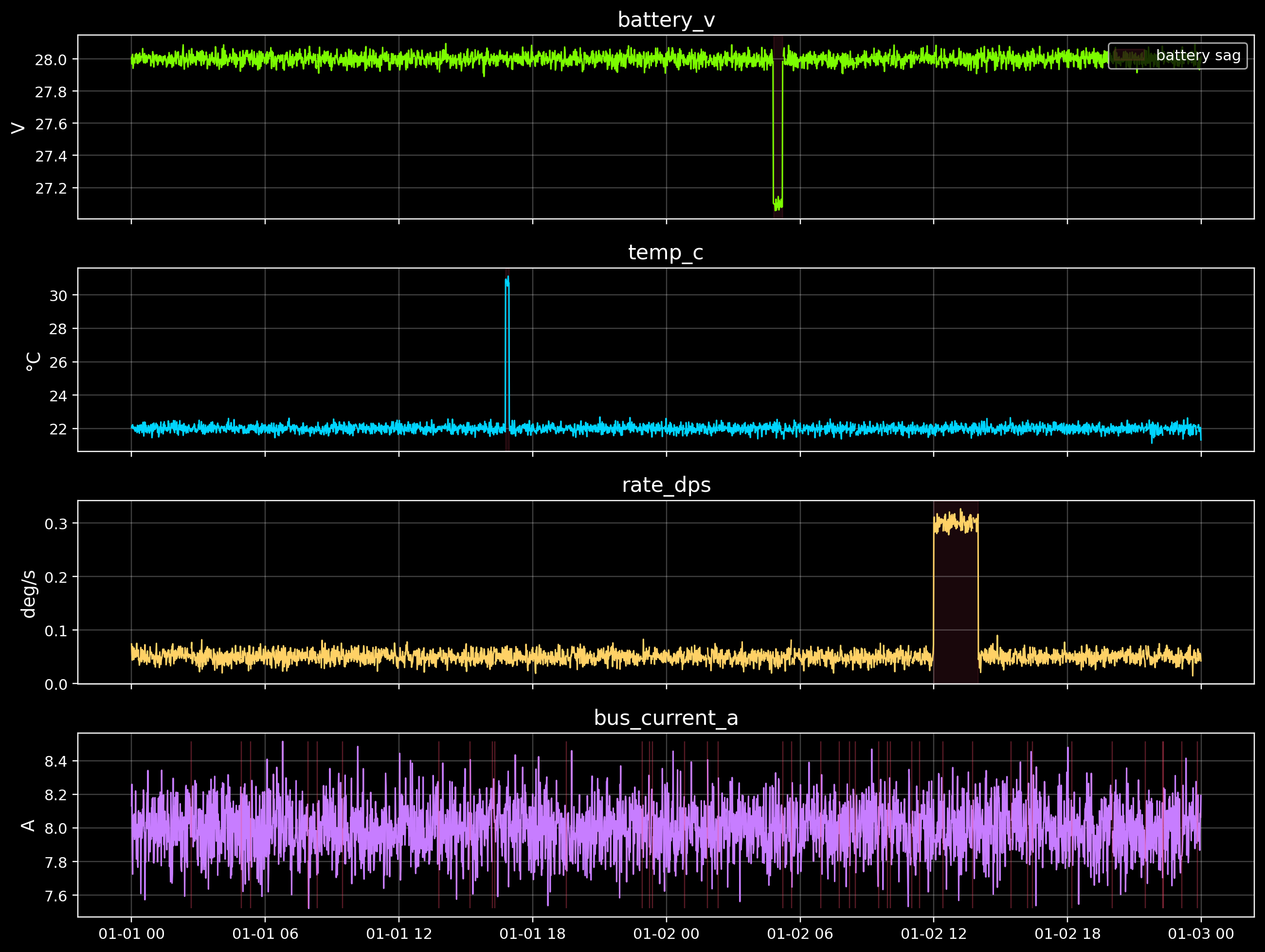
2) Visualize the telemetry (with anomaly windows)

First step in anomaly detection is simple: look at the data.

We’ll plot each signal and mark where we injected the toy anomalies.

def span(ax, start_idx: int, end_idx: int, color: str, label: str):
    ax.axvspan(df.index[start_idx], df.index[end_idx - 1], color=color, alpha=0.10, label=label)


fig, axes = plt.subplots(4, 1, figsize=(12, 9), sharex=True)

axes[0].plot(df.index, df["battery_v"], color=GOOD, lw=1.0)
axes[0].set_title("battery_v")
axes[0].set_ylabel(units["battery_v"])
axes[0].grid(True, alpha=0.25)
span(axes[0], battery_start, battery_end, DANGER, "battery sag")

axes[1].plot(df.index, df["temp_c"], color=ACCENT, lw=1.0)
axes[1].set_title("temp_c")
axes[1].set_ylabel(units["temp_c"])
axes[1].grid(True, alpha=0.25)
span(axes[1], temp_start, temp_end, DANGER, "temp spike")

axes[2].plot(df.index, df["rate_dps"], color="#ffd166", lw=1.0)
axes[2].set_title("rate_dps")
axes[2].set_ylabel(units["rate_dps"])
axes[2].grid(True, alpha=0.25)
span(axes[2], rate_start, rate_end, DANGER, "rate step")

axes[3].plot(df.index, df["bus_current_a"], color="#c77dff", lw=1.0)
axes[3].set_title("bus_current_a")
axes[3].set_ylabel(units["bus_current_a"])
axes[3].grid(True, alpha=0.25)

# Mark missing samples as vertical tick marks on the last plot (gaps matter)
missing_times = df.index[df.isna().any(axis=1)]
axes[3].vlines(missing_times, ymin=df["bus_current_a"].min(), ymax=df["bus_current_a"].max(), color=DANGER, alpha=0.35, lw=0.8)

axes[0].legend(loc="upper right")
plt.tight_layout()
plt.show()

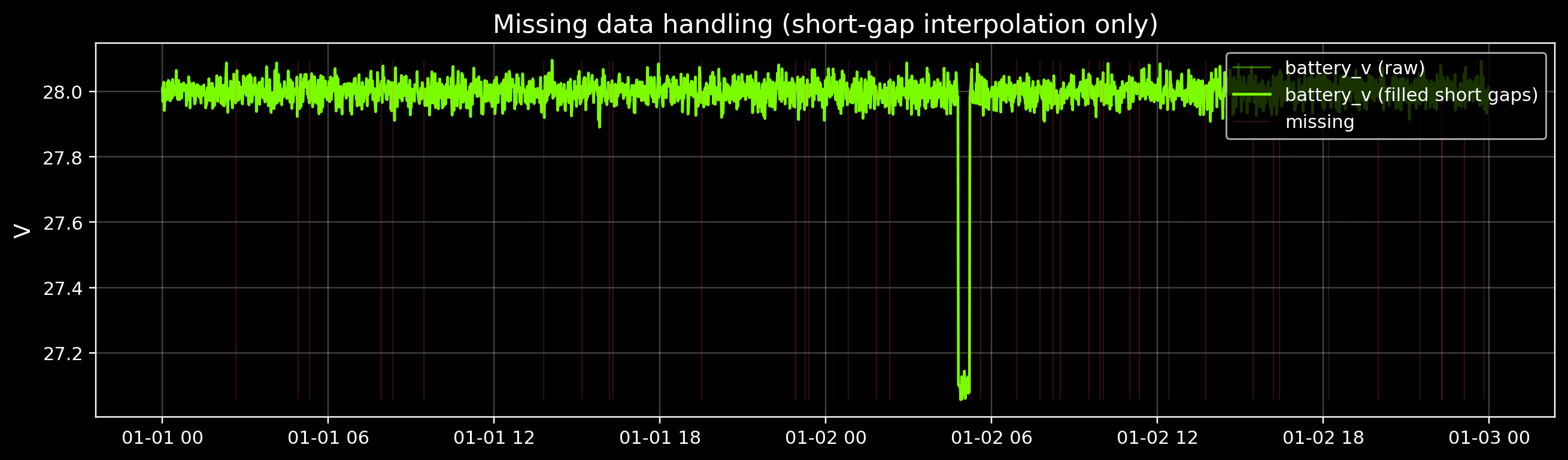
3) Preprocess: handle missing data (carefully)

Missing samples are common in spacecraft telemetry. For most detectors, you have three options:

• Drop missing rows (simple, but you lose time context)
• Forward fill (dangerous if the signal changes quickly)
• Interpolate short gaps (good default for small gaps)

We’ll interpolate only short gaps, and we’ll keep a mask of which timestamps were originally missing.

missing_mask = df.isna().any(axis=1)

# Interpolate only short gaps (up to 3 minutes)
df_filled = df.interpolate(limit=3)

print("Missing timestamps:", int(missing_mask.sum()))
print("Remaining missing after short-gap interpolation:", int(df_filled.isna().any(axis=1).sum()))

# Quick visual: raw vs filled for one signal
sig = "battery_v"
fig, ax = plt.subplots(figsize=(12, 3.6))
ax.plot(df.index, df[sig], color=GOOD, alpha=0.45, lw=1.0, label=f"{sig} (raw)")
ax.plot(df_filled.index, df_filled[sig], color=GOOD, lw=1.5, label=f"{sig} (filled short gaps)")
ax.vlines(df.index[missing_mask], ymin=np.nanmin(df[sig]), ymax=np.nanmax(df[sig]), color=DANGER, alpha=0.18, lw=0.8, label="missing")
ax.set_title("Missing data handling (short-gap interpolation only)")
ax.set_ylabel(units[sig])
ax.grid(True, alpha=0.25)
ax.legend(loc="upper right")
plt.tight_layout()
plt.show()

Missing timestamps: 40
Remaining missing after short-gap interpolation: 0

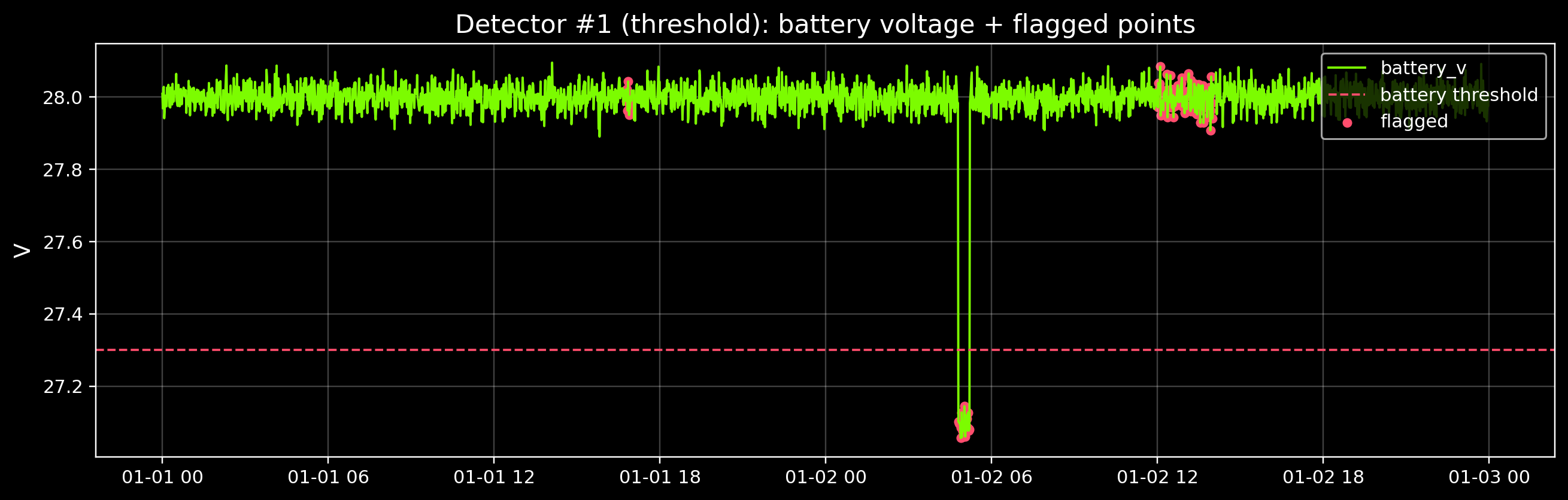
4) Detector #1 — Threshold rules (engineering limits)

Threshold rules are simple and explainable:

• “Battery voltage below 27.3 V is suspicious”
• “Temperature above 27 °C is suspicious”
• “Rate above 0.15 deg/s is suspicious”

Real teams start with these rules because they’re easy to review and audit.

thr = {
    "battery_v_low": 27.3,
    "temp_c_high": 27.0,
    "rate_dps_high": 0.15,
}

pred_threshold = (
    (df_filled["battery_v"] < thr["battery_v_low"])
    | (df_filled["temp_c"] > thr["temp_c_high"])
    | (df_filled["rate_dps"] > thr["rate_dps_high"])
).fillna(False)

print("Threshold flags:", int(pred_threshold.sum()))

# Visualize flags on top of the battery signal (one example)
fig, ax = plt.subplots(figsize=(12, 3.9))
ax.plot(df.index, df_filled["battery_v"], color=GOOD, lw=1.25, label="battery_v")
ax.axhline(thr["battery_v_low"], color=DANGER, lw=1.2, ls="--", label="battery threshold")
ax.scatter(df.index[pred_threshold], df_filled.loc[pred_threshold, "battery_v"], color=DANGER, s=18, label="flagged")
ax.set_title("Detector #1 (threshold): battery voltage + flagged points")
ax.set_ylabel(units["battery_v"])
ax.grid(True, alpha=0.25)
ax.legend(loc="upper right")
plt.tight_layout()
plt.show()

Threshold flags: 155

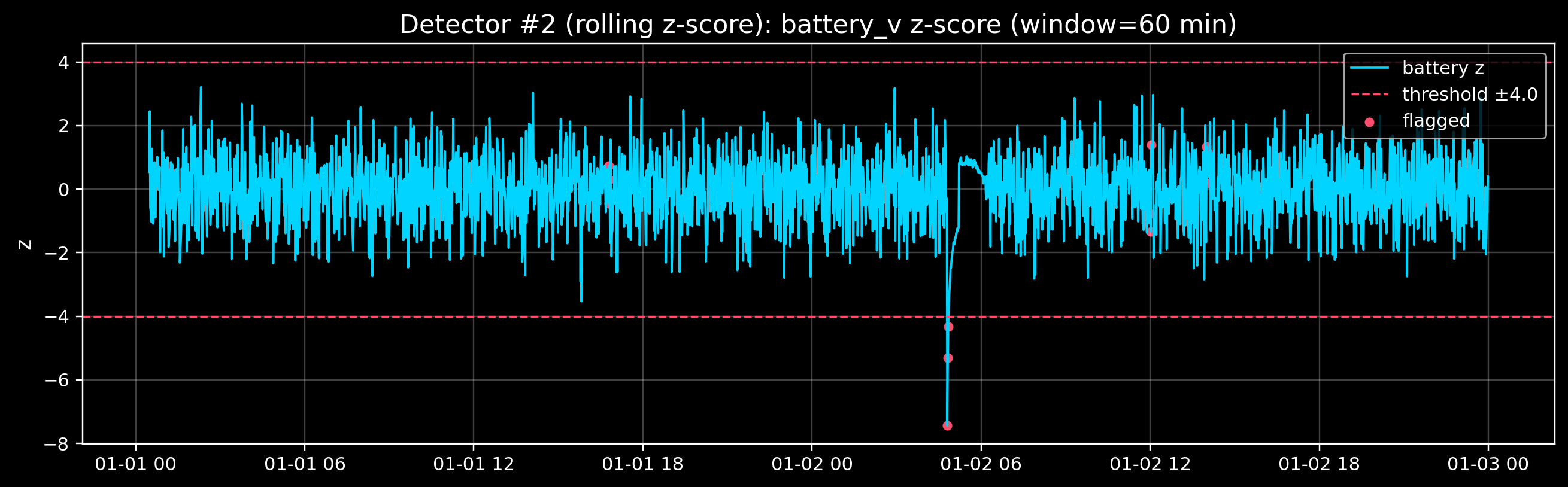
5) Detector #2 — Rolling z-scores (statistical deviation)

A z-score answers: “How many standard deviations away from normal is this sample?”

For time series, we usually compute it relative to a rolling window: - rolling mean - rolling standard deviation

This adapts to slow changes, but it can also hide slow drift (we’ll discuss that later).

def rolling_zscore(x: pd.Series, window: int, min_periods: int = 30) -> pd.Series:
    mu = x.rolling(window=window, min_periods=min_periods).mean()
    sigma = x.rolling(window=window, min_periods=min_periods).std(ddof=0)
    sigma = sigma.replace(0, np.nan)
    return (x - mu) / sigma


window = 60  # 60 minutes
z_batt = rolling_zscore(df_filled["battery_v"], window=window)
z_temp = rolling_zscore(df_filled["temp_c"], window=window)
z_rate = rolling_zscore(df_filled["rate_dps"], window=window)

z_thr = 4.0
pred_roll_z = ((z_batt.abs() > z_thr) | (z_temp.abs() > z_thr) | (z_rate.abs() > z_thr)).fillna(False)

print("Rolling z-score flags:", int(pred_roll_z.sum()))

# Visual: z-score for one signal + flagged points
fig, ax = plt.subplots(figsize=(12, 3.8))
ax.plot(df.index, z_batt, color=ACCENT, lw=1.2, label="battery z")
ax.axhline(+z_thr, color=DANGER, lw=1.1, ls="--")
ax.axhline(-z_thr, color=DANGER, lw=1.1, ls="--", label=f"threshold ±{z_thr:.1f}")
ax.scatter(df.index[pred_roll_z], z_batt[pred_roll_z], color=DANGER, s=18, label="flagged")
ax.set_title(f"Detector #2 (rolling z-score): battery_v z-score (window={window} min)")
ax.set_ylabel("z")
ax.grid(True, alpha=0.25)
ax.legend(loc="upper right")
plt.tight_layout()
plt.show()

Rolling z-score flags: 13

6) Detector #3 — Robust rolling z-scores (median + MAD)

Standard deviation is sensitive to outliers.

A more robust option uses: - rolling median (instead of mean) - rolling MAD (median absolute deviation) instead of standard deviation

This is often better when you expect occasional spikes.

def rolling_mad(x: pd.Series, window: int, min_periods: int = 30) -> pd.Series:
    med = x.rolling(window=window, min_periods=min_periods).median()
    mad = (x - med).abs().rolling(window=window, min_periods=min_periods).median()
    return mad


def robust_rolling_z(x: pd.Series, window: int, min_periods: int = 30) -> pd.Series:
    med = x.rolling(window=window, min_periods=min_periods).median()
    mad = rolling_mad(x, window=window, min_periods=min_periods)

    # Scale MAD to be comparable to std for a normal distribution
    sigma_robust = 1.4826 * mad
    sigma_robust = sigma_robust.replace(0, np.nan)
    return (x - med) / sigma_robust


rz_batt = robust_rolling_z(df_filled["battery_v"], window=window)
rz_temp = robust_rolling_z(df_filled["temp_c"], window=window)
rz_rate = robust_rolling_z(df_filled["rate_dps"], window=window)

rz_thr = 4.0
pred_robust = ((rz_batt.abs() > rz_thr) | (rz_temp.abs() > rz_thr) | (rz_rate.abs() > rz_thr)).fillna(False)

print("Robust rolling flags:", int(pred_robust.sum()))

fig, ax = plt.subplots(figsize=(12, 3.8))
ax.plot(df.index, rz_temp, color="#ffd166", lw=1.2, label="temp robust z")
ax.axhline(+rz_thr, color=DANGER, lw=1.1, ls="--")
ax.axhline(-rz_thr, color=DANGER, lw=1.1, ls="--", label=f"threshold ±{rz_thr:.1f}")
ax.scatter(df.index[pred_robust], rz_temp[pred_robust], color=DANGER, s=18, label="flagged")
ax.set_title(f"Detector #3 (robust z): temp_c robust z-score (window={window} min)")
ax.set_ylabel("z")
ax.grid(True, alpha=0.25)
ax.legend(loc="upper right")
plt.tight_layout()
plt.show()

Robust rolling flags: 98

7) Score the detectors (precision / recall)

Because we injected toy anomalies, we have a ground truth label.

We’ll score detectors on non-missing timestamps and treat “anomaly” as: - battery sag OR temp spike OR rate step

This is simplified, but it teaches the evaluation loop.

y_true = labels["battery_sag"] | labels["temp_spike"] | labels["rate_step"]

# Score only where we actually have data
valid = ~missing_mask.to_numpy()

def score_detector(y_true_bool: np.ndarray, y_pred_bool: np.ndarray, valid_mask: np.ndarray) -> dict:
    y_true_v = y_true_bool & valid_mask
    y_pred_v = y_pred_bool & valid_mask

    tp = int(np.sum(y_true_v & y_pred_v))
    fp = int(np.sum(~y_true_v & y_pred_v))
    fn = int(np.sum(y_true_v & ~y_pred_v))
    tn = int(np.sum(~y_true_v & ~y_pred_v))

    precision = tp / (tp + fp) if (tp + fp) else 0.0
    recall = tp / (tp + fn) if (tp + fn) else 0.0
    f1 = (2 * precision * recall) / (precision + recall) if (precision + recall) else 0.0

    return {
        "tp": tp,
        "fp": fp,
        "fn": fn,
        "tn": tn,
        "precision": precision,
        "recall": recall,
        "f1": f1,
    }


y_pred = {
    "Threshold rules": pred_threshold.to_numpy(),
    f"Rolling z (w={window})": pred_roll_z.to_numpy(),
    f"Robust z (w={window})": pred_robust.to_numpy(),
}

rows = []
for name, yp in y_pred.items():
    s = score_detector(y_true, yp, valid)
    s["detector"] = name
    rows.append(s)

df_scores = pd.DataFrame(rows).set_index("detector")
df_scores[["precision", "recall", "f1"]] = df_scores[["precision", "recall", "f1"]].round(3)

display(df_scores)

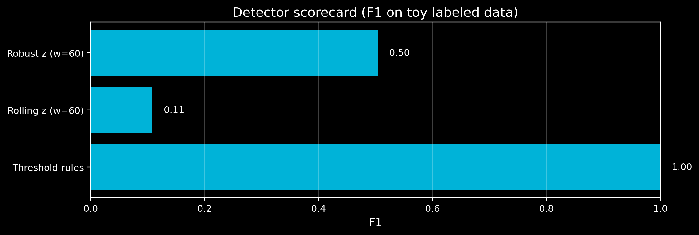
# Visual scorecard
fig, ax = plt.subplots(figsize=(10.5, 3.6))
ax.barh(df_scores.index, df_scores["f1"], color=ACCENT, alpha=0.85)
ax.set_xlim(0, 1)
ax.set_title("Detector scorecard (F1 on toy labeled data)")
ax.set_xlabel("F1")
ax.grid(True, axis="x", alpha=0.25)
for i, v in enumerate(df_scores["f1"].values):
    ax.text(v + 0.02, i, f"{v:.2f}", va="center")
plt.tight_layout()
plt.show()

	tp	fp	fn	tn	precision	recall	f1
detector
Threshold rules	153	0	0	2727	1.000	1.000	1.000
Rolling z (w=60)	9	4	144	2723	0.692	0.059	0.108
Robust z (w=60)	63	34	90	2693	0.649	0.412	0.504

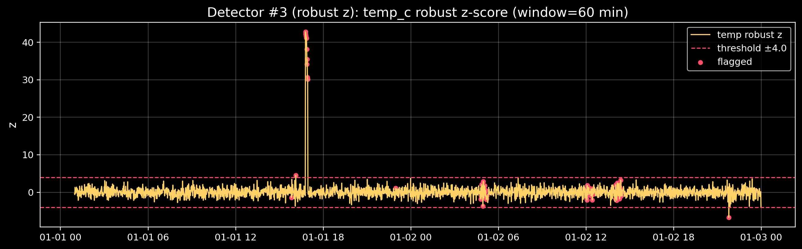
8) What can I do next?

• Exercise A (trade-offs):
  • Change thresholds (thr) and watch precision/recall change.
• Exercise B (window size):
  • Change window from 60 → 20 → 180.
  • When do you start missing the step change? When do false alarms increase?
• Exercise C (missing data):
  • Increase the number of missing samples.
  • What breaks first? (Plots, detectors, scoring?)

Next notebook

In 03_Forecasting_Basics.ipynb, we’ll build simple baselines to predict a time series and quantify error.