Module 4: Human Factors, Regulations, and Space Policy
This notebook explains what astronauts feel during ascent and reentry, and how engineers model it.
What you’ll learn
What g‑load means and how to convert acceleration → g’s
What vibration is (and why resonance can be dangerous)
A simple mass‑spring‑damper model for a crew seat
1) What is “g”?
A g‑load is acceleration measured relative to Earth’s gravity:
1 g = the acceleration you feel standing still on Earth
3 g = three times that load (you feel ~3× heavier)
In code we often convert:
[ = ]
Where (g_0 ,^2).
Code
import numpy as npimport matplotlib.pyplot as plt# Keep visuals consistent with the rest of Rocket Basics "dark_background" )"figure.dpi" : 110 ,"axes.titlesize" : 14 ,"axes.labelsize" : 12 ,"xtick.labelsize" : 10 ,"ytick.labelsize" : 10 ,"legend.fontsize" : 10 ,= "#00d4ff" = "#ff4d6d" = "#7CFC00" = 9.80665 # m/s^2 (standard gravity) print ("Environment ready. Let's talk about human factors." )
Environment ready. Let's talk about human factors.
2) Convert acceleration to g‑load
Engineers and flight controllers talk about g’s because it’s an intuitive “human scale.”
A rocket’s guidance computer works in m/s²
A human experiences the result as g‑load
Let’s implement a tiny helper.
Code
def accel_to_g(accel_m_s2: float ) -> float :"""Convert acceleration magnitude (m/s^2) to g-load.""" return abs (accel_m_s2) / G0# Example: 29.4 m/s^2 is about 3 g print ("29.4 m/s^2 ->" , round (accel_to_g(29.4 ), 2 ), "g" )
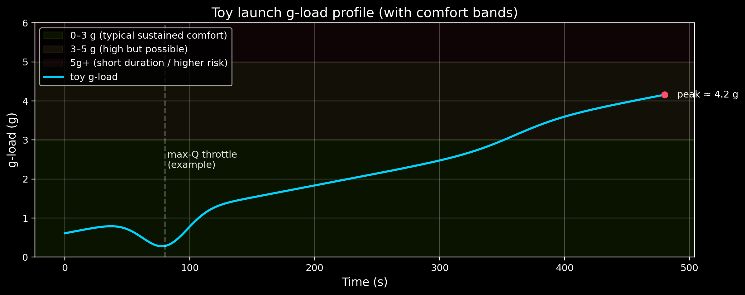
3) A simplified launch “g profile”
Real launch acceleration depends on vehicle mass, throttling, drag, and guidance. But we can still learn a lot from a simplified picture:
Early in ascent, acceleration is modest (vehicle is heavy + drag is high)
As propellant burns off, the vehicle gets lighter, so acceleration tends to rise
Near max‑Q, some rockets throttle to reduce loads
Below is a toy example — not a specific vehicle.
Code
= np.linspace(0 , 480 , 481 ) # seconds # Toy acceleration model (m/s^2): ramp up + a "max-Q throttle dip" + final push = 6.0 + 0.06 * t # slow ramp from ~0.6 g to ~3.6 g over 8 minutes = 8.0 * np.exp(- 0.5 * ((t - 80 ) / 18 ) ** 2 ) # dip centered at ~80 s = 6.0 * (1 / (1 + np.exp(- (t - 360 ) / 20 ))) # late-stage rise = base - max_q_dip + final_push= accel / G0= plt.subplots(figsize= (11 , 4.4 ))# Comfort bands (illustrative; not a medical standard) 0 , 3 , color= GOOD, alpha= 0.08 , label= "0–3 g (typical sustained comfort)" )3 , 5 , color= "#ffd166" , alpha= 0.08 , label= "3–5 g (high but possible)" )5 , 10 , color= DANGER, alpha= 0.06 , label= "5g+ (short duration / higher risk)" )= ACCENT, linewidth= 2.2 , label= "toy g-load" )"Toy launch g‑load profile (with comfort bands)" )"Time (s)" )"g‑load (g)" )True , alpha= 0.25 )# Guide marks 80 , color= "white" , alpha= 0.25 , linestyle= "--" )82 , max (g_load) * 0.55 , "max‑Q throttle \n (example)" , fontsize= 10 , alpha= 0.9 )= float (np.max (g_load))= float (t[int (np.argmax(g_load))])= DANGER, s= 40 , zorder= 5 )+ 10 , max_g, f"peak ≈ { max_g:.1f} g" , va= "center" )0 , max (6 , max_g * 1.15 ))= "upper left" )
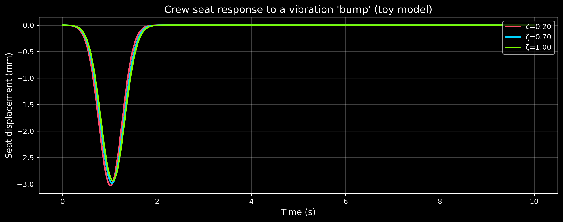
4) Vibration: a seat as a mass‑spring‑damper
A common “first model” for crew comfort is a mass‑spring‑damper system:
[ m, + c, + k,x = F(t) ]
Where: - (x) is seat displacement - (m) is astronaut + seat mass - (k) is stiffness - (c) is damping
Instead of working with (c) directly, we often talk about the damping ratio ():
(< 1): under‑damped (oscillates)
(= 1): critically damped (fastest settling without oscillation)
(> 1): over‑damped (slow return)
Below we simulate a simple “bump” input and compare damping values.
Code
from scipy.integrate import solve_ivpdef seat_response(zeta: float , f_n_hz: float = 5.0 , duration_s: float = 10.0 ):"""Return time + displacement for a 2nd order mass-spring-damper seat model. We model a base-acceleration 'bump' as an input acceleration a(t), and convert it to an equivalent forcing. This is simplified, but it teaches the idea. """ = 2 * np.pi * f_n_hzdef a_bump(t):# Smooth bump (m/s^2) ~0.3 g peak around t=1.0 s return 0.3 * G0 * np.exp(- 0.5 * ((t - 1.0 ) / 0.25 ) ** 2 )def ode(t, y):= y# x¨ + 2ζω_n x˙ + ω_n^2 x = -a(t) = - 2 * zeta * omega_n * xdot - (omega_n** 2 ) * x - a_bump(t)return [xdot, xddot]= np.linspace(0 , duration_s, int (duration_s * 200 ) + 1 )= solve_ivp(ode, (0 , duration_s), y0= [0.0 , 0.0 ], t_eval= t_eval, rtol= 1e-6 , atol= 1e-9 )return sol.t, sol.y[0 ]def plot_seat_responses(zetas):= plt.subplots(figsize= (11 , 4.4 ))= [DANGER, ACCENT, GOOD, "#c77dff" ]for i, z in enumerate (zetas):= seat_response(zeta= z)* 1000 , linewidth= 2.2 , color= colors[i % len (colors)], label= f"ζ= { z:.2f} " )"Crew seat response to a vibration 'bump' (toy model)" )"Time (s)" )"Seat displacement (mm)" )True , alpha= 0.25 )= "upper right" )0.2 , 0.7 , 1.0 ])
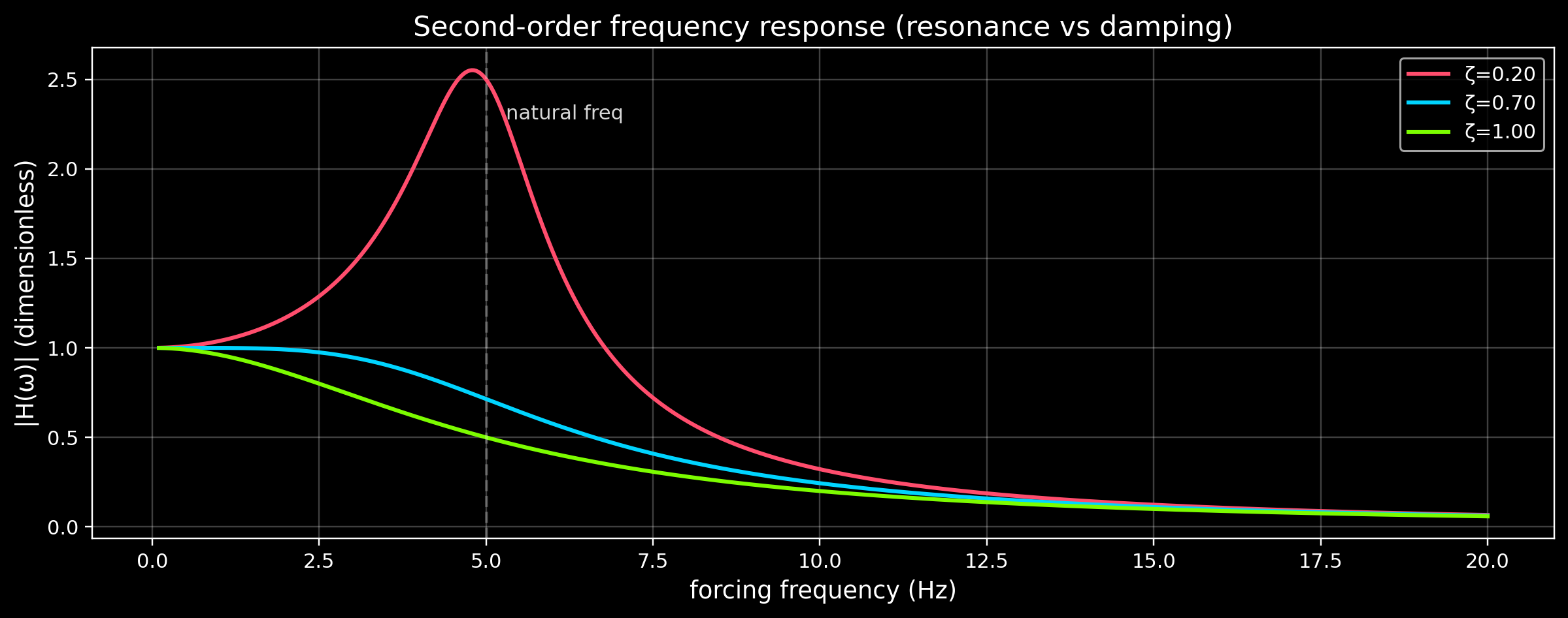
5) Resonance intuition (frequency response)
The scary part of vibration is resonance : if the forcing frequency matches the system’s natural frequency, the response can spike.
A simple second‑order system has a (dimensionless) magnitude response:
[ |H()| = ]
We’ll plot (|H|) for a few damping ratios (). Notice how higher damping reduces the peak.
Code
def frequency_response_mag(freq_hz: np.ndarray, f_n_hz: float , zeta: float ) -> np.ndarray:= freq_hz / f_n_hzreturn 1.0 / np.sqrt((1 - r** 2 ) ** 2 + (2 * zeta * r) ** 2 )= 5.0 = np.linspace(0.1 , 20.0 , 600 )= [0.2 , 0.7 , 1.0 ]= [DANGER, ACCENT, GOOD]= plt.subplots(figsize= (11 , 4.4 ))for z, c in zip (zetas, colors):= frequency_response_mag(freq, f_n_hz= f_n, zeta= z)= c, lw= 2.0 , label= f"ζ= { z:.2f} " )= "white" , alpha= 0.25 , ls= "--" )+ 0.3 , ax.get_ylim()[1 ] * 0.85 if ax.get_ylim()[1 ] > 0 else 1.0 , "natural freq" , alpha= 0.85 )"Second-order frequency response (resonance vs damping)" )"forcing frequency (Hz)" )"|H(ω)| (dimensionless)" )True , alpha= 0.25 )= "upper right" )
6) What can I do next?
Run the full simulator (interactive controls + more context):
cd src/Module_04_Human_Factors/Projects/Crew_Safety_Simulatorpip install -r requirements.txtpython simulator.py
Question to test yourself:
If a capsule experiences (a = 49,^2), what g‑load is that?
Mini exercise:
Change the damping ratio list in the plots. What value gives a “good compromise” between fast settling and low peak response?
If you want to go deeper, look for: - NASA‑STD‑3001 (human systems integration) - Launch & reentry acceleration profiles from public mission reports (NASA, ESA, Roscosmos, CNSA, JAXA)